


Executive Summary
Today’s high performance homes require smart fresh air ventilation and smart comfort conditioning systems that are responsive to the dynamics of human activities. Energy use in yesterday’s era of inefficient homes were dominated by climate variations. Today’s homes are significantly impacted by humans. Average humans do not exist. Proper accounting for human ventilation needs and comfort conditioning preferences requires statistical assessments to design homes that are likely to satisfy most people.
This report presents field data and analyses to define human ventilation and comfort preferences. We use “3 sigma” design to characterize humans. The following summarizes our findings:
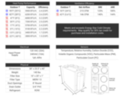
- Online IAQ setpoint information from CERV and CERV2 smart ventilation systems indicate an average setpoint preference of 993ppm for CO2 and total VOCs, with a standard deviation of 190ppm.
- Average fresh air flow rate associated with preferred IAQ setpoint is 24cfm per occupant with a standard deviation of 8.5cfm.
- Residential fresh air ventilation systems, based on 3 sigma design and residence occupancy of 6 to 8 people should have 300cfm of air flow ventilation capability
- Dynamic comfort conditioning loads, such as thermostat setpoint changes, occupant comfort preference variations (eg, inactive versus exercising), and activity changes (eg, cooking) require sufficient comfort conditioning capacity in order to change indoor temperatures within a reasonable time.
- 2 to 3kW (6800 to 10,200Btuh) of heating and cooling capacity are recommended for meeting dynamic comfort conditioning needs based on 3 sigma comfort conditioning load variations from an extensive set of field data collected in 13 identical homes (with non-identical people) over a one year period.
- The human dynamic comfort conditioning load should be added to a home’s design day, climate comfort conditioning needs.
- Increased comfort conditioning capacity can increase house energy efficiency with today’s high performance minisplit heat pumps. Electrical energy efficiency gains of 25% or more are possible when operating two, independent minisplit heat pumps at partial capacity rather than a single heat pump operating at high capacity.
Introduction – Designing Homes for People
We have entered the era in which humans and climatic conditions dominate a home’s energy use. Designing a home’s air quality and comfort for an “average” human results in dissatisfaction, discomfort, and unending callbacks for home designers and contractors. Average humans do not exist!
Statistical characterizations of air quality and comfort preferences are required to design homes for “most” people. Weather variations use “design day” methods for statistical accounting of a location’s climate. For example, Chicago’s 99.6% heating design day temperature is -5F (-20.6C, ASHRAE Handbook of Fundamentals), indicating that 99.6% of the time, air temperature is higher. Design day weather conditions are an example of “3 sigma” design. “Sigma” is the standard deviation of a data set, and 3 sigma variation indicates that a design includes 99.7% of expected variations.
Human air quality and comfort preferences vary among humans, as well as over time for an individual. For example, someone reading a book would likely prefer a warmer environment than someone exercising. An active person can require 10 times more fresh air than someone sleeping. A home’s fresh air ventilation and comfort systems should have dynamic capacities for these human preference variations.
Yesterday’s poorly insulated, leaky, climate-dominated homes masked human air quality and comfort needs. That is, design day heating and cooling methods provided additional capacity for human-based load variations. Climate-based design is no longer adequate in high performance homes for predicting human comfort conditioning and fresh air ventilation requirements. We recommend using 3 sigma design to account for fresh air and comfort conditioning loads caused by human preference variations.
Doorway height design will help us to understand why 3 sigma design is reasonable for human ventilation and comfort preferences. A home builder constructing doorways with the same height as the average height for people will have complaints from 75 to 90% of their homes even though only 50% of the populace is inconvenienced. Using 3 sigma design for air quality and comfort preferences reduces “callback” dissatisfaction.
One would think that highly engineered, architecturally designed commercial buildings satisfy human air quality and comfort preferences, and yet, survey results indicate otherwise. A study of 34,169 commercial building occupants spread over 215 buildings in North America and Finland found widespread dissatisfaction in both air quality and comfort [1]. ASHRAE design standards are based on 20% populace dissatisfaction with air quality and comfort [2]. Only 26% of the surveyed buildings had air quality dissatisfaction less than 20%! And, worse, only 11% of the surveyed buildings had less than 20% thermal discomfort dissatisfaction! Survey respondents reported a self-assessed level of work productivity that correlated with their level of air quality and comfort dissatisfaction, indicating a business cost exceeding the cost to smartly improve ventilation and comfort conditions. It is time to place the human as a priority, and create excellent indoor environments at work, at school, and especially at home where we spend most of our time!
The answer to achieving home occupant satisfaction with air quality and comfort is remarkedly simple. Every residence, single family dwellings and multi-family residences, should be capable of supplying 300cfm of fresh air and have 1 ton of heating and cooling capacity. Even the most perfectly insulated and sealed residence in mild climates should have 1 ton of heating and cooling capacity!
As an added twist, we discuss today’s minisplit heat pumps that operate more efficiently at part load capacity. Designers and builders should consider installing two 1 ton heat pumps even though a climate-based design model might suggest that only a candle’s worth of heat is needed for comfort. Two of today’s high efficiency, minisplit heat pumps operating at half capacity are more efficient than a single heat pump operating at full capacity. And, two units can improve comfort distribution, provide redundancy, and keep your homes’ occupants even happier!
Why 3 Sigma? Door Height Design
If you designed and built single occupancy homes with doorway height for the average human, the door height would be 5’7” [3]. Curiously, more than half of your homes will complain. Today’s typical North American doorway height is 6’8”. Somehow, we have iterated to a door height design that covers 99.8%, or 3 sigma variation of population height [3].
We often hear of “3 sigma” as a design benchmark in which 99.7% of the human population is covered. Door height, whether by statistical analysis or a natural iterative evolution by home builders trying to minimize complaints, is an example of 3 sigma design in which almost all the population would be satisfied with door height. But, why 3 sigma? Wouldn’t 1 sigma design covering 68% of the populace or 2 sigma design that covers 95% of the population be ok?
We use doorways to explore how doorway height impacts complaints. Note that doorway height, air quality, and heating/cooling capacity are examples in which half of the population would be satisfied with “average” conditions. Someone shorter than average is likely to be ok with average doorways. Someone who prefers cooler than average indoor temperatures in the winter and warmer than average in the summer is likely to be satisfied with average heating and cooling capacity design.
Average design will cause household dissatisfaction that is greater than half because households generally have more than one occupant. Some analysis is needed to explain how average doorway heights lead to disproportionate complaint levels.
Doorway height, air quality, and comfort conditioning are a type of problem in which a certain fraction of the population will be satisfied once a level of performance (doorway height, heating capacity, fresh air flow rate) exceeds our need. Shoe size is a different, more complex type of problem. For cases such as shoe size, almost everyone would be dissatisfied with average shoes. Proper shoe design requires a distribution of shoe sizes and shapes that matches a person’s feet, in contrast to air quality and comfort that require a minimum capability to satisfy a range of preferences.
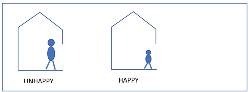
Imagine a house with an average human height doorway. If all homes have one occupant, assuming half of the populace is shorter and the other half is taller than average, we would expect the taller half of the population to be dissatisfied with the doorway. Figure 1 is a schematic of this situation. Yes, there may be some taller than average folks who like bowing down when entering and exiting a house, and there may be shorter than average people who feel claustrophobic with the slightly larger than their height doorway, but these are secondary effects and are not the point of the example. As with coin tossing, an architect or builder may be fortunate that “heads” (short people) comes up 10 times or more in a row, resulting in very few doorway complaints. In the long run, however, statistical averages will result in 50% of home occupants complaining about door height.
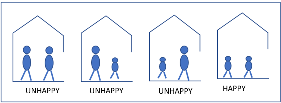
Adding a second occupant to our home creates four occupant combinations. Two tall people, a short person and a tall person, a tall person and a short person, or two short people. Figure 2 shows these situations. Three of the four situations will result in unhappy occupants due to doorway height, indicating that 75% of homes with 2 occupants will complain!
Extending this line of thought to a home with 3 occupants, we would find that 87.5% of homes would be likely to complain about door height. For homes with 4 occupants, 93.8% of the homes would complain. As we reach 8 occupants, 99.6% or virtually all homes would complain about door height. In other words, as occupancy levels increase, the likelihood that a household will complain about door height rapidly increases.
Average occupancy in US homes is 2.5 people, perhaps indicating that 75 to 87% of the homes would be dissatisfied with average design. However, the complaint issue should be expanded beyond a single house because it doesn’t matter that if we are discussing an individual house or a group of homes and apartments. A developer building a few hundred homes will have never-ending doorway height complaints, and few buyers or tenants. And, of course, a home with shorter than doorway height occupants are likely to have taller than doorway height friends that visit, making it likely that they will complain, too. It only takes a few people to have a 99.6% dissatisfaction rate!
We can reduce complaints and callbacks by flipping the situation around and designing doorway heights such that 0.3% of the populace are taller than standard doorways. Similarly, air quality and comfort complaints can be reduced to lower levels if we design homes to accommodate 99.7% of populace preferences. But, what are those preferences and what are the costs to meet those needs? Build Equinox field data allows us to define air quality and comfort preferences. The cost to satisfy a 3 sigma spread of population driven air quality and comfort preferences is reasonable.
Home Air Quality Preferences
We first characterize residential air quality preferences because it is relatively straightforward. The basic questions we wish to answer are the following: If a home’s occupants can choose their air quality, what would they select, and what is the associated ventilation airflow rate? Data related to residential, human-controlled indoor air quality preferences have not been available until the introduction of CERV and CERV2 smart ventilation units.
Occupants in CERV and CERV2 smart ventilated homes choose their home’s air quality by selecting a carbon dioxide and total VOC (Volatile Organic Compounds) concentration setpoint. Whenever CO2 or VOC concentrations exceed an occupant chosen setpoint, CERV units switch to fresh air ventilation until air pollutants are reduced 100ppm below the setpoint threshold. The total VOC concentration scale we use correlates a human’s VOC output in relation to a human’s CO2 output. Ideally, a human whose respiration results in a CO2 concentration of 1000ppm would also result in a correlated total VOC concentration of 1000ppm. Non-human VOC sources added to an indoor environment increase total VOC readings above CO2 levels. When humans are the primary source of CO2 and VOCs, or in buildings with indoor combustion sources (eg, gas cooking), CO2 may be the dominate indoor pollutant.
Our second generation CERV2 smart ventilation units increased fresh air ventilation flow to a maximum of 300 to 400cfm from the first generation unit’s 200 to 250cfm maximum airflow rate. Air flow in second generation CERV2 units were increased based on multiple factors:
- Doubling current recommended (ASHRAE 62.1 and 62.2) ventilation from an average of 20cfm per person to 40cfm per person reduces airborne disease transmission (flu and colds) with an effectiveness equivalent to that of the flu vaccine and improves human productivity, sleep and cognition.
- By 2050, increased atmospheric carbon dioxide will require double the fresh air ventilation flow rate required in 1950 for the same indoor carbon dioxide concentration level.
- An increased fresh air flow rate decreases the time required to exhaust indoor pollutants, allowing the CERV2 unit to spend more time in recirculation mode, which is essential for:
- Filtering and reducing indoor air particulate concentrations
- Utilizing fresh air “stored” in unoccupied regions of a home
- Unifying comfort conditions
- CERV2 air flow capability of 300 to 400cfm matches air flow rates for 1 ton ducted minisplit heat pumps, allowing ductwork to be efficiently utilized for both fresh air ventilation and comfort conditioning.
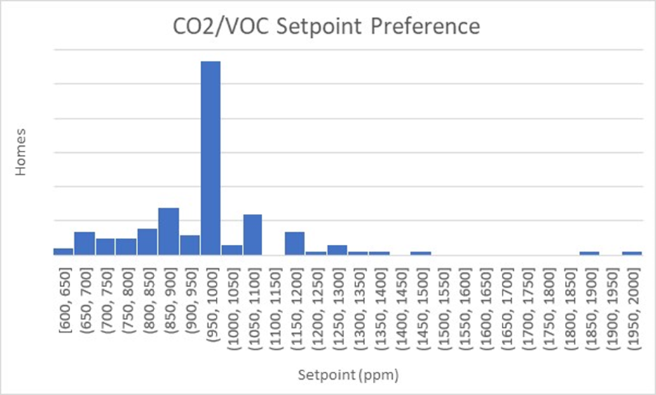
Figure 3 shows IAQ setpoint preference variations for 135 homes with CERV and CERV2 ventilation units. CO2/VOC setpoint conditions were collected at an instant of time (in November 2019). The average setpoint is 993ppm with a standard deviation of 190ppm from the average setting. Build Equinox presets default CERV2 IAQ setpoint to 1000ppm, which is approximately equivalent to the pollutant exposure one experiences with ASHRAE ventilation standards. We suspect that many homeowners tend to leave pollutant setpoints at our default settings and that if we were to reduce the default setting (eg, Equinox House uses 850ppm setpoint) that many homes would use that setting.
CERV and CERV2 owners choose whether to stay connected to the internet or to operate without online connectivity. The data is therefore representative of those CERV and CERV2 homes in which the homes have chosen to be connected online. CERV and CERV2 online data is not sold nor shared, and CERV/CERV2 users can request deletion of data from Build Equinox at any time.
The importance of the online CERV/CERV2 Community cannot be overstated. An individual’s data can help them to improve their wellbeing. Collectively, an individual’s data contributes to our overall understanding of how to efficiently improve our sense of well-being. That is, my data can help you and your data can help me. It is in this spirit that all CERV data from Equinox House (my home) can be viewed online, as well as live operating conditions in Equinox House.
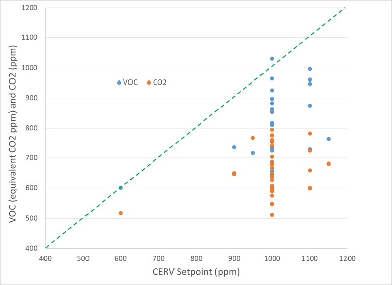
Figure 4 shows average CO2 and total VOC levels for 34 all-electric, high performance homes in Vermont over a 5 month period (January through May, 2017) relative to each home’s chosen pollutant setpoint. In general, most homes have an average indoor pollutant concentration level below the setpoint level. Some homes with significant pollutant generation rates have pollutant concentrations similar to the setpoint level. Homes that have pollutant concentrations at or above the setpoint level are homes with significant generation rates of indoor pollutants and have significant (perhaps continuous) fresh air ventilation requirements.
The data in Figure 4 shows most of the 34 homes are dominated by VOC levels rather than CO2 concentration. When correlated VOC concentration levels exceed CO2 concentrations, sources of VOCs in addition to human generated VOCs are present in a home. We note that human production of VOCs varies widely relative to their CO2 output. Perhaps, someone eating large quantities of garlic compared to someone on a bland diet, or just variations of one’s metabolism and microbiome are responsible?
Historical CERV data allows homeowners to determine whether VOCs are from humans or from other pollutant generating sources by observing whether VOC concentrations stay high in the absence of occupation, or tend to decrease in concert with CO2 decreases when occupants leave the home. In the latter case, the VOC-to-CO2 ratio is a characteristic of the home occupant pollutant generation levels while the former indicates some other VOC source is present. Locating the source of non-human VOCs is desirable for reducing ventilation needs and pollutant levels.
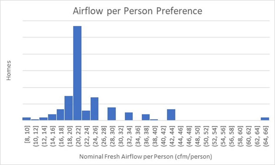
Figure 5 is a distribution plot of nominal fresh air flow rates per person among the 135 CERV/CERV2 homes discussed in Figure 3. The nominal fresh air flow rate is the air flow required to maintain the IAQ setpoint with a person whose metabolism produces 0.04kg/hour of CO2, representative of sedentary (office work activity) metabolism. Different metabolism levels, or non-human pollutant generating activities (gas cooking, furniture off-gassing, cleansers, fragrances, etc) alter fresh air flow rate to keep pollutant concentrations below the setpoint. For example, a person with twice the activity level of a sedentary adult would require twice the fresh air flow rate to maintain the same pollutant concentration.
The average fresh air flow rate per person based on an average setpoint of 990ppm is 24cfm per person, or 20% greater than the common 20cfm per person rule-of-thumb. The standard deviation is +/-8.5cfm per person, for a 3 sigma variation of 25.5cfm per person. From our previous discussion of designing for 99.7% of the populace, the data indicates that a fresh air ventilation system should have nearly 50cfm per person fresh air flow capability.
A CERV2, with 300 to 400cfm of ventilation air flow capability, is sufficient for 6 to 8 people based on the most stringent (50cfm per person) IAQ preference. Therefore, in addition to the other cited reasons for the second generation CERV2 unit’s fresh air flow capability, the CERV2 encompasses 3 sigma IAQ preferences of 99.7% of home occupants. 300 to 400cfm ventilation air flow capability also dovetails nicely with air flow rates for a 1 ton heat pump, allowing comfort conditioning and fresh air ventilation to operate in a synergistic manner within a common duct distribution system.
Transient Home Heating and Cooling Effects
Indoor environments are not static! A home’s indoor environment is a dynamic balance of many factors that are continually pushing and pulling a home away from one’s desired comfort conditions. An important reason for minimum heating and cooling capacities are transient heating and cooling effects. Variations of human occupancy, human activities, solar inputs, outdoor ambient conditions, and changes in occupant preferences all contribute to variations of heating or cooling to keep a house comfortable.
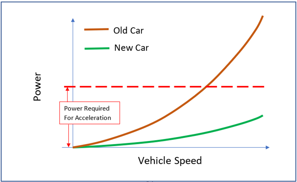
The horsepower needed to drive yesteryear’s inefficient automobiles at high speed on interstate highways was also enough power to accelerate during start-n-stop driving. Today’s streamlined, efficient cars do not need as much power for high speed driving, but still need power for accelerating from traffic stops. Figure 6 is a schematic of automobile horsepower needs relative to power needed for acceleration. A highly streamlined, efficient car with just enough horsepower for steady driving will create road rage as the car slowly creeps to highway speed. Drivers who would like to go faster will also be upset at the lack of horsepower to drive faster than average.
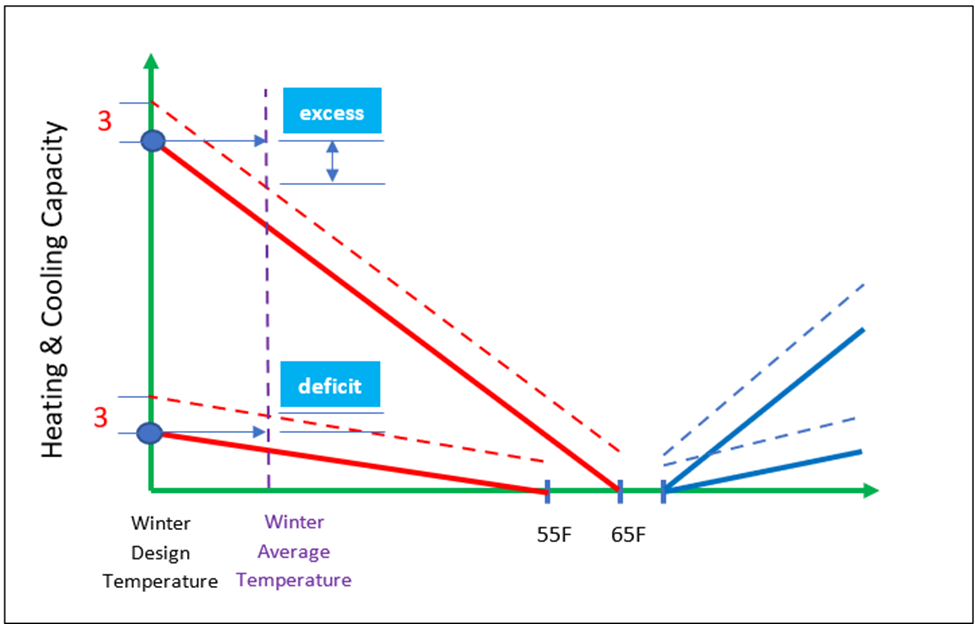
High performance homes are analogous to automobiles. We need enough heating and cooling capacity to “accelerate” a home to different comfort conditions. Figure 7 is a schematic of heating and cooling capacity requirements for a conventional home and a high performance home. Heating and cooling capacity specifications are generally based on a climate-based design day calculation with an average human load effect.
The dashed lines sketched on Figure 7 represent the upper 3 sigma upper bounds for heating and cooling capacity deviations from “average” conditions. The upper solid and dashed lines represent a conventional house with 3 to 4 times the comfort capacity needs of a high performance home. Viewing the heating side of Figure 7, a conventional home’s statistical load variations are smaller than the excess capacity built into design day modeling. That is, the difference between a design day heating requirement and a location’s average winter day’s heating requirement is greater than the 3 sigma statistical heating load variation.
The lower set of lines in the Figure 7 representing a high performance home show how design day predictions of heating and cooling loads are no longer sufficient to meet the dynamic 3 sigma heating and cooling load variations. The difference between design day capacity predictions and average climate capacity requirements are less than the dynamic, 3 sigma capacity variation requirements. The era of high performance homes has moved us to a situation where human impact on comfort conditioning capacity must be accounted for in order to meet home occupant comfort expectations.
We can get an idea of transient heating and cooling load requirements using a simple analytical model (details of the model are included in Appendix A). The thermal mass of a home relative to the comfort conditioning capacity determines the time required to change a home’s indoor temperature. Our ASHRAE Journal article from March 2011 presents field data characterizing the thermal mass of a home as a “time constant”, or number of hours required for a home to cool down to approximately 2/3’s of the way from an initial indoor temperature to the outdoor temperature without active heating.
Equinox House is a thermally massive house with a time constant of 100 hours, compared to a more conventional home’s time constant of 30 hours or less. Note that Equinox House does not have any extra mass added to make it thermally massive.
Assume we have a house with an average indoor temperature of 68F (20C) and an outdoor temperature of 32F (0C). Also, assume the house is a high performance home similar to Equinox House (2100sqft ranch, slab-on-grade with overall transfer coefficient, UA = 360kJ/K-h; thermal time constant = 100hours) and has 3kW (10,600Btu/h) of heating capacity. With full heating capacity, the house will increase 0.16F in 1 hour, 1.6F in 10 hours, and 3.6F in 24 hours. Doubling the heating capacity to 6kW (21,200Btu/h) increases indoor temperature by 0.7F in 1 hour, 7F in 10 hours, and 15F in 24 hours.
The difference between 3kW and 6kW of heating capacity is very significant in terms of changing a home’s interior temperature. Even though 3kW may be sufficient to meet design day heating capacity predictions, the home will not have sufficient capacity to have any noticeable change in indoor temperature over the course of several hours. A home with 6kW of heating capacity will noticeably change indoor temperature over the course of a few hours. The cost to add more heating and cooling capacity is small ($1 per square foot for 1 ton of capacity for many locations). And, as we will discuss later, in today’s world of inverter drive (speed control) compressors and fans, operating at partial heating and cooling capacity increases system efficiency!
Statistical Description of House Heating and Cooling Requirements
Field data from real people in real homes is necessary for determining dynamic heating and cooling capacity requirements. We examine data collected from 13 “identical” Vermod homes over a year. Details of the homes and extensive field data tables on IAQ, comfort conditions, and energy usage (cooking, hot water, laundry, plug loads, etc) are included in a Build Equinox report [4]. We re-examine some of the characteristics of four of the homes in terms of indoor temperatures and daily energy usage. Statistical analyses are then applied to the daily heating and cooling loads to define the 3 sigma boundaries that define minimum heating and cooling needs due to dynamic house load fluctuations.
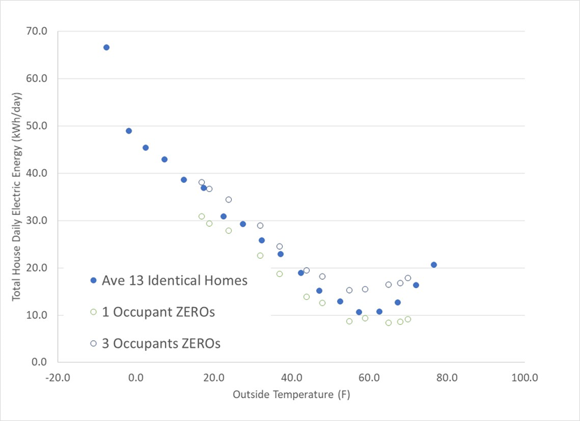
Figure 8 shows ZEROs (Zero Energy Residential Optimization software) electrical energy usage predictions for Vermod homes with 1 occupant and 3 occupants. ZEROs is an online, free-to-use house design model developed by Build Equinox. The Vermod report includes details of house construction characteristics (insulation, windows, infiltration, etc). Average occupancy of the Vermod homes is 2.5 people. The Vermod house data shown in Figure 8 is the average of data for all 13 homes, sorted into 5F outdoor temperature bins. The agreement between ZEROs and the averaged Vermod home energy performance is excellent.
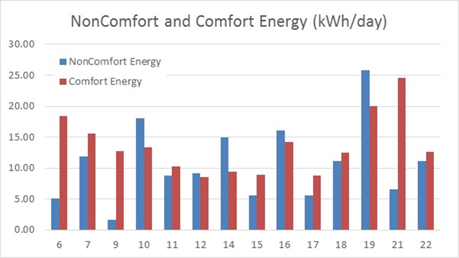
Figure 9 shows annual electrical energy usage of the 13 Vermod homes. House energy is separated into electrical energy for comfort conditioning electrical and for other (hot water, cooking, laundry, TVs, etc). The variation of annual energy usage among homes is very large, and is not strongly correlated to occupancy, although there are various energy uses, such as hot water and laundry, that do strongly correlate with occupancy (see the Vermod report for further details). Note that house numbers are not successive and do not with “House 1” because other non-Vermod homes were also part of the study.
House 22 in Figure 9 is the average of all 13 Vermod homes. As with people and weather, one can average home energy usage, but there are no average houses. Without finer detail, it is very clear that some homes use much more energy than average while others use much less. Any home requiring more than average energy would be quite dissatisfied if they were restricted from enjoying some activity due to an enforced limitation on their energy usage. Five of the 13 homes required more energy for non-comfort conditioning uses, five homes used more energy for comfort conditioning, and three homes were in reasonable balance. All homes are located in Vermont, one of the most severe and longest winter seasons in the US, indicating that less harsh climates are likely to experience even higher non-comfort energy to comfort conditioning energy ratios.
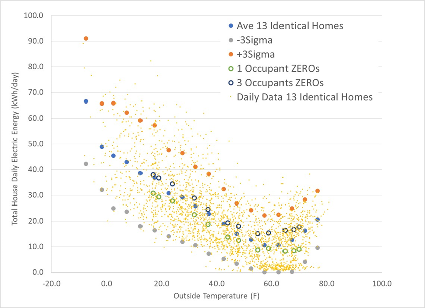
Figure 10 repeats Figure 8 with the addition of daily electrical energy data for all 13 homes. Figure 10 clearly shows that many of the 13 homes regularly require significantly more electrical energy than “average”. In fact, a majority of the homes regularly exceed the average home’s energy requirements. More than half of the homes are likely to express dissatisfaction if their home is restricted to an average daily energy usage.
Also plotted on Figure 10 are data points representing 3 sigma boundaries for the data. The 3 sigma boundaries are approximately +/-15kWh per day from average usage, or approximately 625W of continuous power usage. If a home was continuously operating at the upper boundary, an additional 5500kWh per year (~$600-700 extra utility bill) above average is used. Note that House 19 was approximately 20kWh per day higher than the overall house average, so exceptions to 3 sigma occur.
The variation of energy performance among these homes must be kept in perspective. The average Vermod house performance exceeds passive house performance standards by 20%, which is very difficult to achieve in smaller homes in harsh climates. Even though House 19 has an average energy use of 45kWh per day compared to the house average energy usage of 25kWh per day, the annual energy usage (16,425kWh/year) is low compared to a conventional home.
The temptation to throw out “outlier” data points should be avoided. Assuming there are no problems with the data acquisition equipment, outliers (both good and bad) are opportunities to learn. House 19, for example, has 5 occupants and exceptionally high level of cooking energy. On a per person basis, House 19 energy usage is very low!
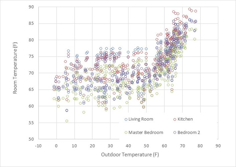
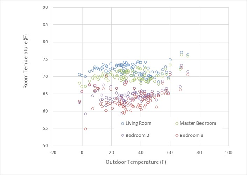
Figures 11-14 show indoor temperature variations as a function of outdoor temperature for 4 of the Vermod homes. These homes were selected as examples to display a variety of characteristics. House 6 (Figure 11) is a home in which the occupants tend to keep the whole home comfortable during the winter, however, they do not use air conditioning during the summer. During winter, indoor temperature varies from 60 to 75F, with an average of 68F. Various dynamic house processes, such as cooking, thermostat changes, and occupant activities contribute to the variations. Interestingly, the home occupants must not be sensitive to high indoor temperatures. With 70 to 80F outside temperatures, indoor temperatures reached 85 to 90F without air conditioning. Similar to wearing a winter coat in the summer, a highly insulated home restricts transfer of indoor generated heat from cooking, occupants, plugs, etc to the outside. The occupants most likely opened windows and doors to vent as well as possible, however, approaching outdoor temperatures with natural cooling is difficult.
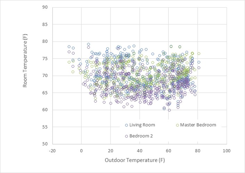
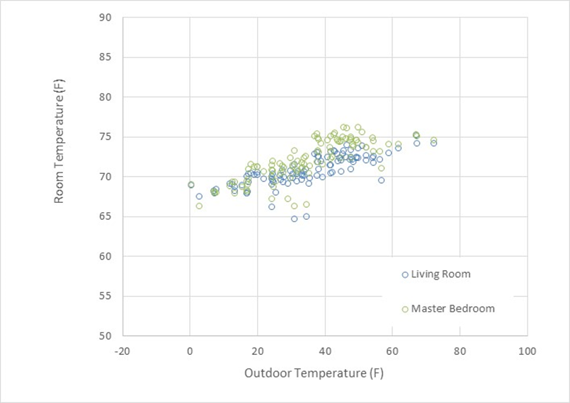
The occupants of House 7 (Figure 12) have similar winter comfort preferences as House 6, with dynamic house temperature variations between 60 and 75F, and an average indoor temperature of 68F. Unlike House 6, House 7 occupants also prefer the same indoor conditions during the summer.
House 15 is a low energy user, with low comfort and non-comfort energy usage. Bedrooms 2 and 3 are significantly colder during the winter, indicating that the occupants have closed air vents and doors to those rooms. Elevated trends in temperature during summer conditions indicate a reluctance to use air conditioning. House 17 is also a low energy user similar to House 15. Notice that both Houses 15 and 17 have much less variation of indoor temperature in contrast to House 7. House 7’s annual energy usage is similar to the “average” home energy usage. House 7’s dynamic variations are large, with significant excursions in temperature due to cooking, occupant activities, etc.
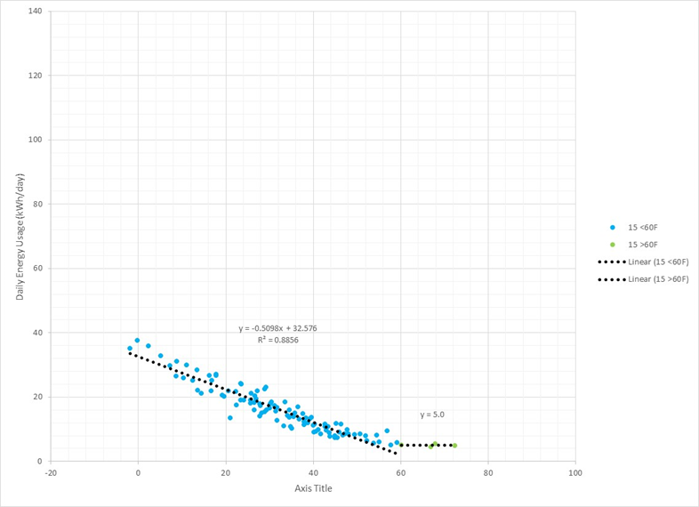
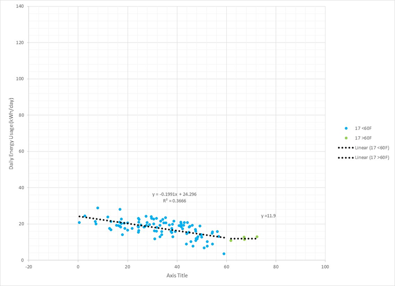
Figures 15-18 show daily energy usage variations for Houses 6, 7, 15 and 17. Houses 6 and 7 have significant winter variations, while Houses 15 and 17 have low energy usage variations. Perhaps the occupants in Houses 15 and 17 are frequently out of the house, and tend to eat meals outside the home in comparison to Houses 6 and 7? During the summer, House 6 has very low energy with no air conditioning as previously mentioned. Perhaps (but unknown to us), the home was vacant during the summer, with comfort conditioning systems turned off? Switching comfort conditioning systems off during vacancy periods can allow mold to grow and should be avoided. Minimal energy is required to keep an unoccupied, high performance home conditioned.
The energy required to keep House 7 comfortable is shown in Figure 16. Comfort is important and has value. Comfort is important for human productivity, sleep, healing, and relieves stress on the elderly and infirm. The cost for comfort during the summer in House 7 is approximately 8kWh per day, or less than $1 per day of additional electricity usage.
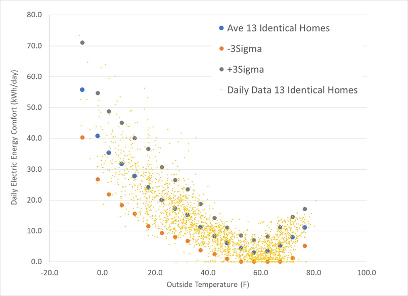
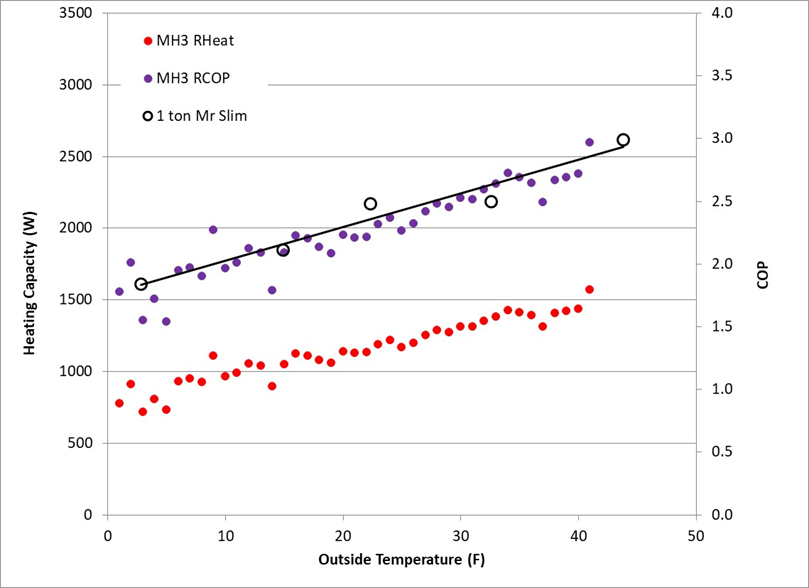
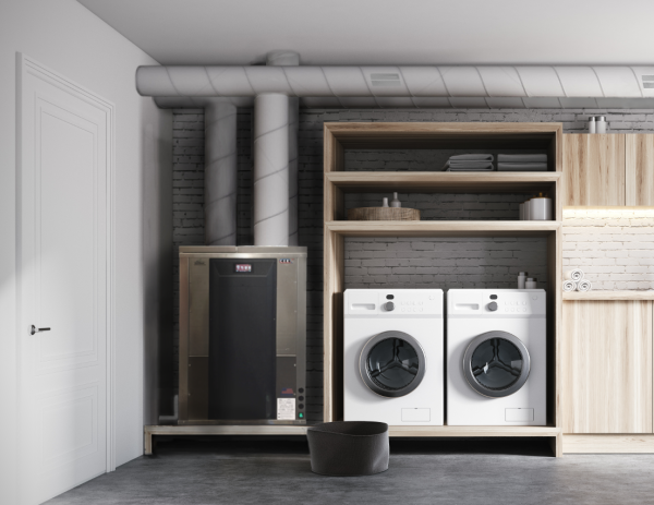
Figure 19 shows daily electrical energy usage for comfort conditioning in the 13 Vermod homes. Vermod homes included in the study are heated and cooled with a combination of minisplit heat pump (1 ton “Mr Slim” Mitsubishi Ductless Hyperheat) and first generation CERV smart ventilation units. CERVs use a heat pump to exchange energy between fresh air and exhaust air streams when energy exchange is beneficial. When fresh air ventilation is not needed, the CERV operates in a recirculation mode, contributing its heating or cooling/dehumidification capacity for comfort conditioning. Figure 20 shows a plot of a CERV unit’s heating capacity during recirculation mode. Also plotted is the CERV unit’s COP (Coefficient of Performance) and the COP for a 1 ton Mitsubishi minisplit heat pump.
CERV heating and cooling capacities are approximately 1/3 of a ton in comparison to the nominal 1 ton minisplit heat pump capacity. Under typical circumstances, the CERV spends 80% of the time in recirculation and 20% in fresh air ventilation. Heating and cooling contributions of the CERV and minisplit heat pump depend on the thermostat settings for each unit. For example, if the CERV has a winter heating thermostat temperature setting of 68F and the minisplit heat pump is set at 70F, the minisplit heat pump will contribute most of the heat. If the settings are reversed, the CERV will contribute as much as it can to heating needs, with any additional heating supplied by the minisplit heat pump. Because the COPs of the minisplit and CERV are similar, the source of heating is not significant, allowing us to analyze both comfort conditioning systems together.
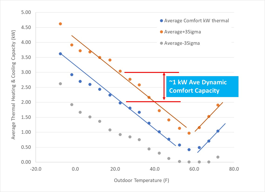
Figure 21 converts electrical energy usage for comfort conditioning into estimated daily heating and cooling capacity requirements. The +/-10 to 12kWh per day 3 sigma variation of comfort conditioning electrical energy usage in Figure 19 is an average of +/-1kW (3400Btu/h) of dynamic heating and cooling needs as shown in Figure 21. Note that daily “average” heating and cooling capacity variations are more likely 2 to 3kW conditioning capacity active over a shorter time period. That is, if the dynamic comfort conditioning usage occurred within 12 hours, 2kW (6800Btu/h) of heating/cooling capacity rather than 1kW of capacity is needed. Similarly, if the dynamic conditioning capacity occurred within 8 hours, 3kW (10,200Btu/h) of dynamic capacity is needed.
How can it be that dynamic loads are at least 1kW, and most likely 2 to 3kW in a home? A human’s average metabolic heat output is only 100W, and most design manuals list average plug loads and appliance loads to be 100 to 200W. Ovens and cooktops are capable of 4 to 5kW of heat addition to a home. 100sqft of unshaded windows with 50% SHGC (Solar Heat Gain Coefficient) facing the sun on a clear day can add 5kW of heat, which is more than enough to play havoc with comfort during both summer and winter. Homes with pets and kids that regularly open doors (and leaving them open) impact a home’s energy load. Thermostat setbacks and daily variations in occupant thermostat setting preference cause increased heating and cooling capacity needs as previously discussed.
Recommended Design Approach for 3 sigma Comfort Conditioning Capacity
Our field data indicates that homes have a daily electric energy variation of 10 to 12 kWh per day for comfort conditioning relative to the average comfort conditioning load at any outdoor temperature. This electric energy variation indicates a comfort conditioning capacity need of 1 to 3kW (approximately 1/3 to 1 ton of capacity). Our experience suggests that 1 ton (3 to 4kW, or 12,000Btu/h) is a good base level of heating and cooling capacity for every home, regardless of location.
The dynamic comfort conditioning load effects are primarily due to human occupancy and activities. We expect comfort conditioning variations observed in Vermod homes are valid for other high performance homes, however, this is an area in which additional field data from a variety of homes in a variety of climate regions are desirable. Our personal experience indicates high performance homes with a minimum of 1 ton of heat pump capacity have more satisfied occupants than homes with minimal heating capacity. And, we find home occupants with no active cooling or dehumidification capacity are very likely to regret the absence of summer comfort conditioning. One does not need to use their excess “horsepower”, but it is there when you want it, and over the lifetime of any home, it is likely that some future occupants will want cooling and dehumidification.
We know we are going against the grain and current desire of high performance home designers and builders by advocating a minimum comfort conditioning capacity in all homes. A 1 ton minisplit for a 2000sqft, high performance home, similar to Equinox House (which has design day heating and cooling loads of 1 ton) should have an installed cost of $2000 to $3000, or a cost of $1 to $1.5 per square foot. In combination with a smart ventilation system and heat pump water heater (including distribution ductwork), a high performance home’s “mechanicals” have a combined cost of ~$10,000, or $5 per square foot for a 2000sqft home. Note that commercial and institutional comfort conditioning and ventilation systems cost $100 per sqft of building floor area (while still failing to achieve a healthy, comfortable and satisfying indoor environment)!
Increased Capacity Equals Increased Efficiency!
Imagine walking down the aisles of a home construction conference exposition hall and finding a booth in which the product representative told you they are releasing a premium heat pump system that outperforms today’s already very efficient heat pumps by 25%. Few opportunities exist for increasing energy efficiency in today’s high performance homes. Additional insulation, better house sealing methods, and improved windows are unlikely to increase energy efficiency by this amount. And, additional efforts in these areas will most likely be uneconomical due to the law of diminishing returns.
Increasing heat pump efficiency reduces comfort conditioning electrical energy usage directly, and effectively discounts the cost of heating and cooling loads due to insulation levels, infiltration, windows, appliance usage, and all other activities that impact comfort conditioning loads.
A 25% gain in heat pump performance already exists and is available today, but very few recognize it because the gain comes from an unexpected direction; doubling the heating and cooling capacity of a home’s comfort conditioning system! If your home requires 1 ton of capacity to cover design day weather and dynamic human loads, put in 2 tons. If your home has a design day load of 2 tons, consider adding 3 to 4 tons of heat pump capacity. Nobel Laureate Richard Feynman noted that as complex as physics seems, it all boils down to F=ma; but you must know it very, very well. Similarly, significant gains in heat pump performance have been under our noses for some time, but requires knowing heat pump characteristics very well.
We have already discussed how two, independent 1 ton ductless minisplit heat pumps operating at half capacity are more efficient than a single 1 ton heat pump operating at full capacity (see our June 2018 Minisplit Mania report). This observation is the result of understanding that today’s inverter drive (speed control) heat pumps operate more efficiently at lower capacity settings.
It is understandable that oversizing heat pump capacity and causing them to operate at lower capacity seems contrary to the experience of many in the HVAC field. And, it is likely that if you ask home designers or HVAC professionals about this, you may be told it is not true. But, it is true, and it is not based on magic or wishing-and-a-hoping, but physics.
Yesterday’s “bang-bang” (on-off) controlled heating and cooling systems operate less efficiently at part loads due to transient losses of continuously starting and stopping a unit. Speed control allows systems to operate continuously at the needed capacity. For heat pumps operating at partial capacity, the important effect is a reduction of temperature differences in its heat exchangers, which thermodynamically, is a reduction of inefficiency (entropy generation). Our Minisplit Mania report discusses this effect, and demonstrates that it exists in real systems through an assessment of several ductless heat pumps and from detailed laboratory data.
Demand for minisplit heat pumps is rapidly growing due to their exceptional performance (SEER > 20, HSPF >10), quietness, ease-of-installation, and ease-of-use. North American preference seems to be trending toward “ducted” rather than “ductless” heat pumps, and manufacturers are responding by developing more ducted offerings. Fujitsu has had a low temperature, high performance ducted version of their popular minisplit heat pump for a few years, and Mitsubishi plans to release a ducted version of their popular “Hyper Heat” (full capacity operation down to -13F) minisplit heat pump in 2020.
Laboratory tests at Build Equinox with a 1 ton, Fujitsu ARU12RLF ducted minisplit heat pump demonstrates this effect. Operating the ducted minisplit at high capacity with 32F outside ambient and 67.5F indoor temperature, the unit produced 6.2kW (21.1kBtuh) of heat output with 2.03kW of system power for a COP (Coefficient of Performance, ratio of heat output to power input) of 3.05. Reducing the heat pump’s capacity to lower stage heating under the same indoor and outdoor conditions produced 4.1kW (14.1kBtuh) of heat output with 1.00kW of power for a COP of 4.1.
The ratio of low capacity heating COP to high capacity heating COP is 1.34, or 34% better performance! The ratio of low capacity to high capacity COPs varies with indoor and outdoor conditions, but is significant over a broad range of heating and cooling conditions. In addition to the performance gains, two or more independently operating heat pumps add flexibility for meeting occupant comfort preferences, reduced response time for changes of indoor conditions, and redundancy.
“Multi-head” minisplit heat pumps will not provide the same efficiency gains, and may drop overall efficiency. Multihead units share one outdoor heat exchanger unit, restricting efficiency gains possible with independent, single head units connected to individual outdoor units. Our experience has shown the installed cost difference between two independent, single head units and a single, two-headed unit of the same capacity are negligible. In addition to efficiency gains of independent minisplit units, we prefer independent units for redundancy and control flexibility. Residential multihead heat pumps require all indoor heads to be set for a common mode of heating or cooling. Independent units allow each unit to be operated as desired. In one of our projects, three 1 ton minisplits were installed for the “her” area, “his” area, and common area of the home. Her and his areas differed by 10F in comfort preference, sometimes requiring heating in one and cooling in the other! Basement to second floor thermal stratification can also cause significant conditioning variations.
Cost is always a consideration, and in this case, an additional 1 ton minisplit adds $1500 (check online for direct sale prices) with $500 to $1000 for installation expense (see our news article on minisplit heat pump installation). Is an additional $1 to 2 per sqft worth the additional expense for increased energy efficiency, improved comfort control, and system redundancy? That’s a decision for homeowners. In our case, the answer was yes. Equinox House enjoys exceptional, efficient comfort control all year long with its two 1 ton ductless minisplit heat pumps. You don’t have to take my word for it. Review more than 4 years of Equinox House IAQ (CO2 and total VOCs) and comfort (indoor temperature and humidity) from CERV-ICE (CERV-Intelligently Controlled Environment), our online monitoring and control dashboard included with all CERV2 smart ventilation systems.
References
[1] C. Huizenga, S. Abbaszadeh, L. Zagreus and E. Arens, “Air Quality and Thermal Comfort in Office Buildings: Results of a Large Indoor Environmental Quality Survey”, Proceedings of Healthy Buildings 2006, Lisbon,Vol. III, 393-397, 2006.
[2] Seichi “Bud” Konzo, “The Quiet Indoor Revolution”, University of Illinois press, 1996.
[3] “Anthropomorphic Reference Data for Children and Adults: United States, 2011-2014”, Vital Health and Statistics Series 3, Number 39, August 2016, Centers for Disease Control, Nat’l Center for Health Statistics, US Dept of Health and Human Services.
[4] T. Newell, “13 CERV Vermod Homes: Keeping Occupants Healthy, Comfortable, and Energy Efficient”, Build Equinox research report, June, 2016.
[5] ZEROs, cloud-based, free-to-use Zero Energy Residential Optimization software, by Build Equinox.
[6] T. Newell and B. Newell, “Thermal Mass Design: Solar NZEB Project”, ASHRAE Journal, March 2011.
Appendix A – Transient Heating and Cooling Capacity Model
A “zero order” model (no geometrical dimensions) characterizing a home’s thermal mass effects is useful for examining transient heating and cooling characteristics of a home. For a home with known comfort conditioning capacity, insulation/infiltration, and mass characteristics, a change of indoor temperature from and initial indoor temperature is predicted as:
T – Ti = (Q/UA – (Ti – Ta)) x (1 – exp(-t/ Ƭ))
Where T = indoor temperature at a future time
Ti = initial indoor temperature
Ta = outdoor ambient temperature
Ƭ = house time constant = mc/UA
~100hours
t = time
Q = heating (positive) or cooling (negative) capacity
UA = overall house transfer coefficient (including house infiltration)
~100W/K = 360kJ/K-h (Equinox House)
mc = house mass-heat capacitance product or energy storage characteristic
~36,000kJ/K (Equinox House)
Equinox House is a thermally massive home with a time constant of 110 hours. No extra mass was added to Equinox House beyond that required for foundation and structure. Judicious design of insulation, sealing, and windows are key factors determining a home’s thermal mass. Typical home thermal mass ranges from 25 hours to 100 hours.
The red term in the above relation represents the temperature change possible from the initial condition while the blue term represents the time required to reach a desired change of temperature.